Your warehouse holds thousands in dead inventory while your bestsellers sit empty.
Sound familiar? You’re not alone. Most retailers face this costly paradox that destroys cash flow, frustrates customers, and keeps business owners awake at night, wondering why they can’t get inventory right.
But here’s what the most successful companies know: inventory forecasting eliminates this chaos entirely.
Instead of guessing what to order, you’ll predict demand with mathematical precision. Instead of reactive scrambling, you’ll operate with strategic confidence. Instead of choosing between stockouts and overstock, you’ll achieve that sweet spot where customer demand meets perfect inventory levels.
This comprehensive guide transforms you from inventory victim to inventory master.
What you’ll learn

Core forecasting formulas that calculate exactly what you need, when you need it

Proven forecasting methods and when to use each one

Step-by-step implementation process you can start using immediately

Advanced techniques for handling seasonality, new products, and promotional spikes
TL;DR:
Key takeaways

Inventory forecasting is the most effective way to prevent stockouts and reduce carrying costs

Accurate forecasting requires clean historical data and the right formulas

Combining manual methods with software can optimize your entire supply chain
What is inventory forecasting?
Inventory forecasting is the data-driven process of estimating how much stock you’ll need over a future period so you can meet customer demand without over-ordering. It blends historical sales, lead time, seasonality, and market trends to calculate optimal reorder points, safety stock, and purchase quantities.
At its core, inventory forecasting is a critical process for predicting future inventory needs to meet customer demand perfectly. It’s the difference between running a reactive business that constantly scrambles to keep up and operating a strategic enterprise that stays ahead of market fluctuations.
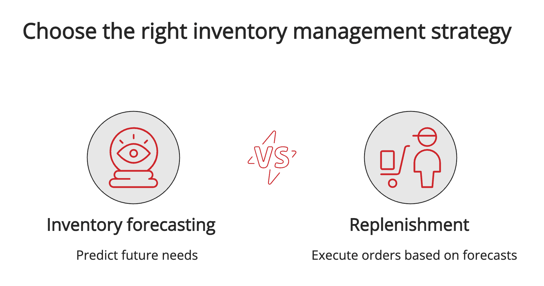
Inventory forecasting vs. replenishment
Inventory forecasting is the analytical process of predicting what you’ll need based on data and trends. Demand forecasting serves as a key input to inventory forecasting, helping you understand customer purchasing patterns. Replenishment is the operational act of ordering products based on your forecasting insights.
Think of it this way: forecasting tells you what to buy, and replenishment is when you actually buy it.
Why it matters: 6 quantifiable benefits
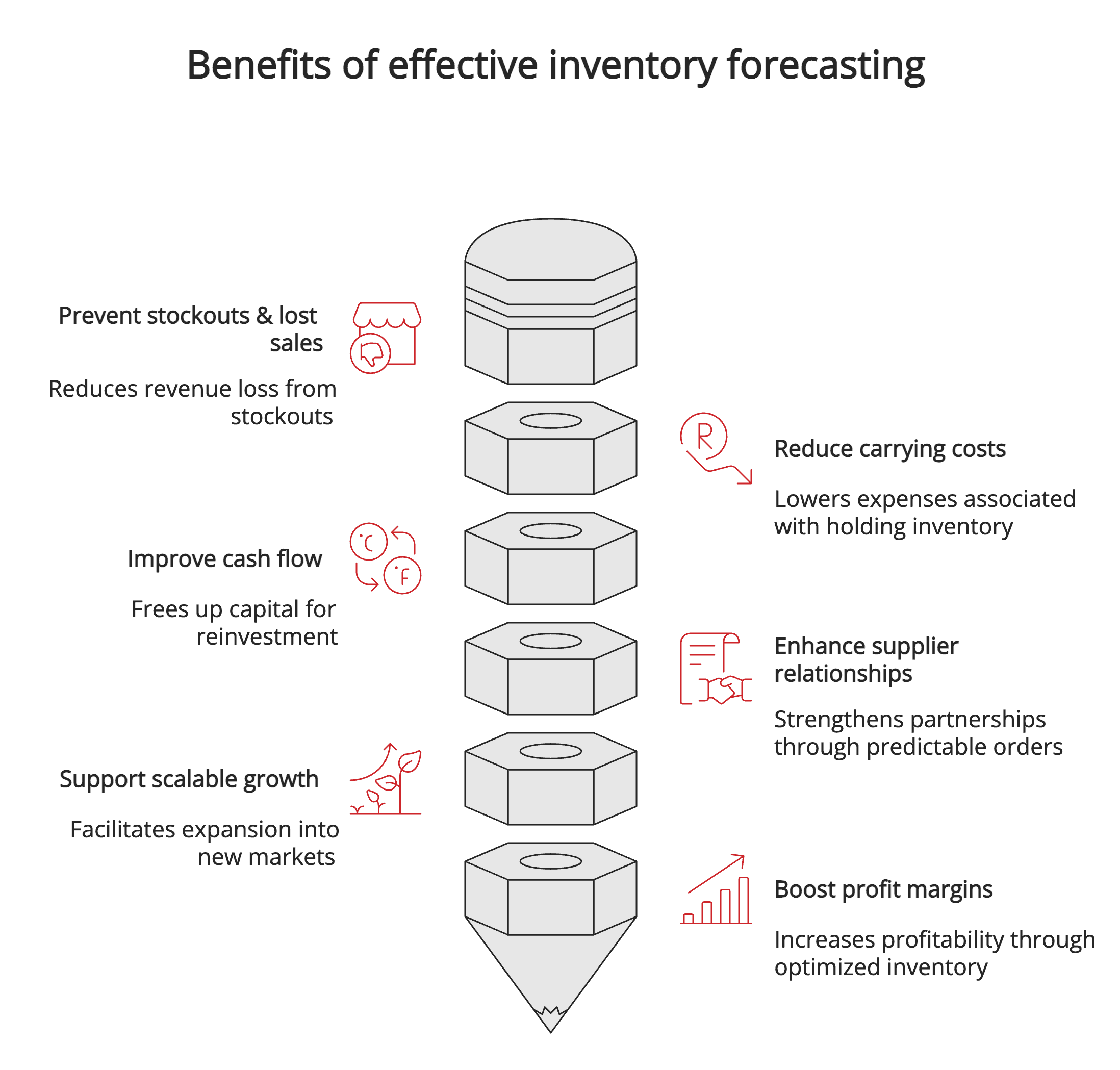
Effective inventory forecasting delivers measurable improvements across your entire operation:
Prevent stockouts & lost sales: Stockouts cost retailers an average of 4% of annual sales, and up to 71% of shoppers will defect to a competitor if an item is out of stock.
Reduce carrying costs: Carrying costs can consume 15-35% of your inventory’s value annually. Accurate forecasting prevents overstock situations that tie up capital unnecessarily.
Improve cash flow: By avoiding excess inventory, you free up capital that can be reinvested in growth, marketing, or new product development.
Enhance supplier relationships: Consistent, predictable orders based on solid forecasting help you negotiate better terms and build stronger partnerships.
Support scalable growth: As you expand into new markets or channels, forecasting provides the framework to scale inventory management efficiently.
Boost profit margins: Reduced waste, fewer markdowns, and optimized inventory levels directly improve your bottom line.
Key metrics & formulas you’ll use
This section forms the technical foundation of any accurate forecast. While the math might seem complex initially, these formulas become your most valuable tools for making data-driven inventory decisions.
Each formula serves a specific purpose in building your complete forecasting picture, and mastering them gives you unprecedented control over your inventory levels.
Sales velocity vs. average sales
Sales velocity measures how quickly products move through your inventory over a specific period, while average sales provides a baseline consumption rate.
The formula:
Sales velocity = Total units sold ÷ Number of days
Average sales = Total units sold ÷ Number of periods
Breakdown of inputs:

Total units sold: Actual quantity moved during the measurement period

Number of days: Length of measurement period in days

Number of periods: Count of measurement intervals (weeks, months, etc.)
Simple worked example: Blue t-shirt sales over 30 days: 150 units

Sales velocity = 150 ÷ 30 = 5 units per day

Average sales (weekly) = 150 ÷ 4.3 weeks = 35 units per week
Lead time & lead time demand
Lead time represents the total time from placing an order until inventory becomes available for sale. Lead time demand calculates how much you’ll sell during this waiting period.
The formula:
Lead time demand = Sales velocity × Lead time (in days)
Breakdown of inputs:

Sales velocity: Daily sales rate from the previous calculation

Lead time: Days from order placement to inventory availability
Simple worked example: Using our blue t-shirt with 5 units daily sales velocity and 14-day lead time: Lead time demand = 5 × 14 = 70 units
Lead time includes all delays: supplier processing, manufacturing, shipping, and your receiving time. Track each component separately to identify improvement opportunities.
Economic order quantity (EOQ)
EOQ determines the optimal order size that minimizes total inventory management costs by balancing ordering costs against holding costs.
The formula:
EOQ = √(2 × Demand × Ordering cost ÷ Holding cost per unit)
Breakdown of inputs:

Demand: Annual units sold

Ordering cost: Fixed cost per purchase order

Holding cost per unit: Annual cost to store one unit
Simple worked example: Blue t-shirt annual demand: 1,800 units, ordering cost: $50, holding cost: $2 per unit EOQ = √(2 × 1,800 × 50 ÷ 2) = √90,000 = 300 units per order
Reorder point (ROP)
Reorder point triggers new orders to ensure you never run out of stock while accounting for lead time and demand variability.
The formula:
ROP = Lead time demand + Safety stock
Breakdown of inputs:

Lead time demand: Units needed during replenishment period

Safety stock: Buffer inventory for demand/supply variations
Simple worked example: Blue t-shirt lead time demand: 70 units, safety stock: 25 units ROP = 70 + 25 = 95 units
Safety stock
Safety stock protects against stockouts caused by demand spikes or supply delays. This buffer inventory level ensures customer satisfaction even when forecasts are imperfect.
The formula:
Safety stock = (Max daily sales × Max lead time) – (Avg daily sales × Avg lead time)
Breakdown of inputs:

Max daily sales: Highest single-day sales recorded

Max lead time: Longest replenishment period experienced

Average figures: Typical sales and lead time values
Simple worked example: Blue t-shirt max daily sales: 8 units, max lead time: 18 days, averages: 5 units/16 days safety stock = (8 × 18) – (5 × 16) = 144 – 80 = 64 units
Inventory turnover & days of stock
Inventory turnover measures how efficiently you convert inventory into sales, while days of stock shows how long current inventory will last.
The formula:
Inventory turnover = Cost of goods sold ÷ Average inventory value
Days of stock = (Current inventory ÷ Sales velocity)
Breakdown of inputs:

Cost of goods sold: Annual COGS from financial statements

Average inventory value: Mean inventory value over the period

Current inventory: Units on hand today
Simple worked example: Blue t-shirt COGS: $18,000, average inventory value: $3,000, current stock: 200 units
01
Inventory turnover = $18,000 ÷ $3,000 = 6 times per year
02
Days of stock = 200 ÷ 5 = 40 days remaining
ALERT: The inventory forecasting formula you choose depends on your business model, but combining multiple approaches gives you the most accurate predictions. Never rely on a single metric.
4 core inventory forecasting methods
The most effective forecast combines multiple inventory forecasting methods depending on your product lifecycle stage, data availability, and market conditions. Understanding when and how to apply each forecasting method gives you the flexibility to adapt your approach as circumstances change.
Each forecast model serves distinct business scenarios, and mastering these approaches transforms you from reactive ordering to strategic inventory planning. The key is knowing which method works best for your specific situation and how to combine them for maximum accuracy.
Time-series forecasting
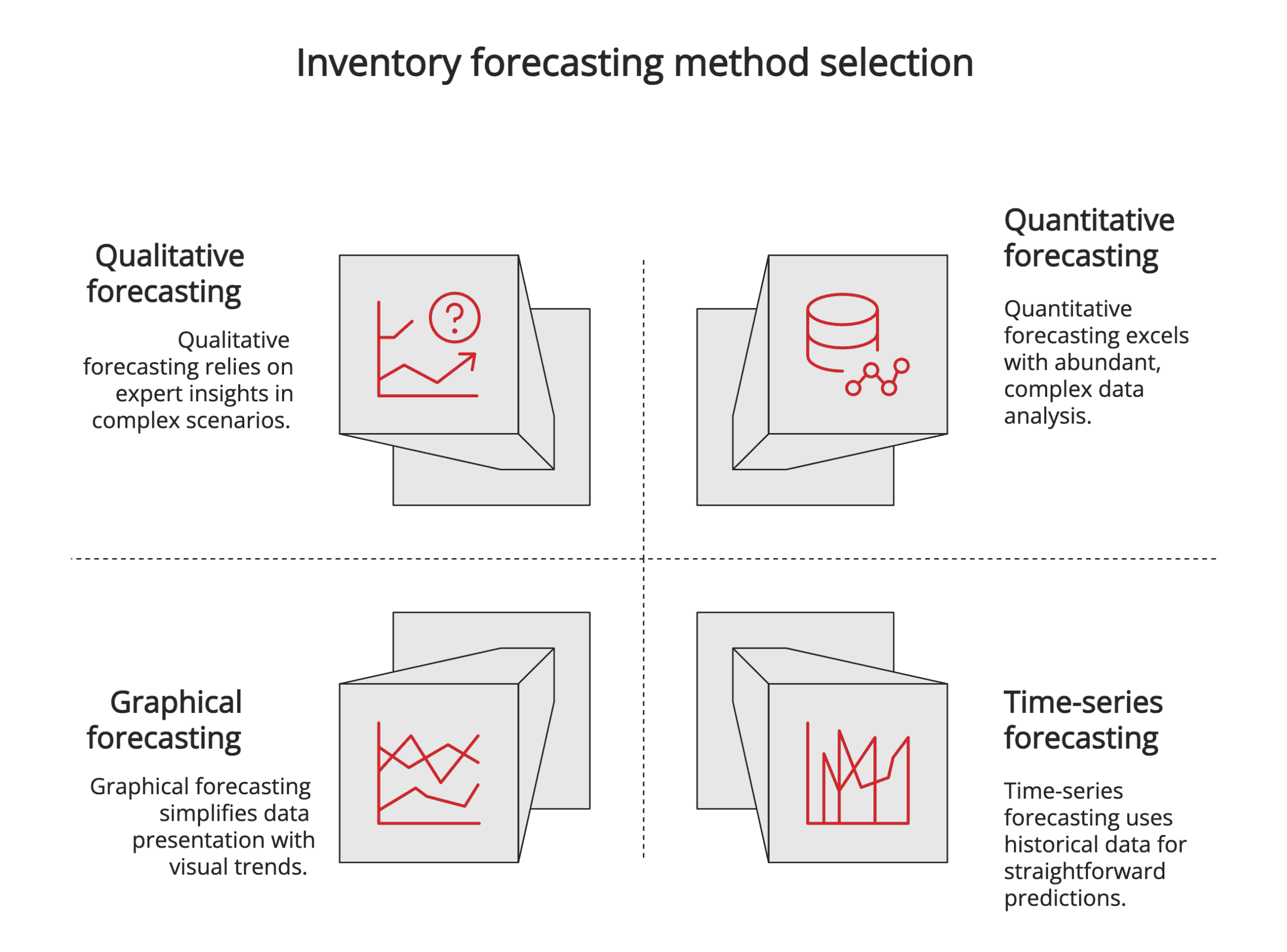
Time-series forecasting analyzes historical sales patterns to project future demand trends. This quantitative approach works best for established products with consistent sales history and clear seasonal patterns.
Best for: Mature products with 12+ months of clean sales data. Strengths: Mathematically precise, identifies trends and seasonality. Limitations: Assumes past patterns will continue
This forecast model becomes particularly powerful when you have stable demand patterns and minimal market disruption. The mathematical precision helps eliminate guesswork from your inventory control decisions.
Graphical forecasting
Graphical forecasting involves plotting historical data visually to identify trends, cycles, and anomalies. This method excels at communicating forecasts to stakeholders and spotting patterns that pure numbers might miss.
Best for: Presenting forecasts to management and identifying visual trends. Strengths: Easy to understand, reveals data stories clearly. Limitations: Subjective interpretation, less precise than mathematical models
Visual analysis often reveals insights that complex algorithms miss, making it a valuable complement to quantitative forecasting methods.
Qualitative forecasting
Qualitative forecasting relies on expert opinion, market research, and industry knowledge rather than historical data. This approach becomes essential when launching new products or entering untested markets.
Best for: New product launches, market disruptions, and insufficient historical data. Strengths: Incorporates market intelligence and expert insights. Limitations: Subjective, potentially biased, difficult to standardize
Quantitative & time-series forecasting
Quantitative forecasting uses statistical models and algorithms to analyze large datasets and identify complex patterns. This forecast model delivers the highest accuracy when you have abundant, clean historical data.
Best for: High-volume businesses with extensive sales history. Strengths: Handles complex variables, most accurate with sufficient data. Limitations: Requires statistical expertise, needs large datasets
When to combine methods (decision matrix)
| If your situation is… | Then use this method… |
|---|---|
| Launching a brand new product | Qualitative forecasting |
| Selling a stable, mature product | Trend & Quantitative forecasting |
| Planning for holiday season | Trend forecasting + Qualitative adjustments |
| Limited sales history | Graphical + Qualitative forecasting |
| Complex seasonal patterns | Quantitative + Time-series models |
Start with the simplest method that fits your data, then layer in complexity as your forecasting capabilities mature. The most successful businesses use multiple inventory forecasting methods simultaneously to cross-validate their predictions and build confidence in their inventory planning decisions.
4-step inventory forecasting process (with templates)
This systematic approach transforms inventory forecasting from overwhelming guesswork into a manageable, repeatable process. Following these steps ensures consistent results and builds confidence in your forecasting capabilities over time.
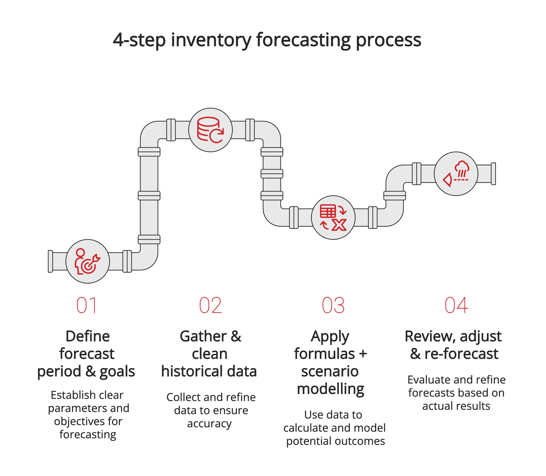
1) Define forecast period & goals
Start by establishing clear parameters for your forecasting initiative. Choose a specific timeframe that aligns with your business cycles—typically 90 days for operational planning or 12 months for strategic decisions.
Set measurable objectives like “reduce stockouts by 15%” or “improve inventory turnover by 20%.” These concrete targets guide your methodology selection and help measure success.
2) Gather & clean historical data
Quality data forms the foundation of accurate forecasting. Remove anomalies like one-time bulk orders, product launches, or major promotional spikes that don’t represent normal demand patterns.
Focus on collecting at least 12-24 months of sales history, supplier lead times, seasonal factors, and any external variables that influence demand. Document your data sources and cleaning decisions for future reference.
Stocktaking accuracy directly impacts forecast reliability. Even small inventory discrepancies compound over time, leading to major forecasting errors.
3) Apply formulas + scenario modelling
This is where the technical work happens. Input your clean data into the formulas from the previous section, starting with basic calculations like sales velocity and building toward more complex metrics like safety stock requirements.
Create multiple scenarios (optimistic, realistic, pessimistic) to understand the range of possible outcomes. Test how changes in key variables affect your final forecasts.
PRO TIP: Download our free Excel template to streamline your calculations and reduce errors. The template includes all formulas pre-built with scenario planning tools.
4) Review, adjust & re-forecast
Inventory forecasting is a continuous improvement process, not a one-time calculation. Track your forecast accuracy by comparing predictions against actual sales, then adjust your methodology based on what you learn.
Schedule regular review cycles—weekly for fast-moving items, monthly for standard products. Document what works and what doesn’t to build institutional knowledge over time.
When sharing forecasts with partners, accuracy becomes critical for successful relationships. Learn how to choose a 3PL that can work effectively with your forecasting data.
Handling seasonality, new products & promotions
Standard forecasting models break down when faced with irregular patterns, new launches, or promotional spikes. These exceptions require specialized approaches that combine mathematical rigor with business judgment.
Seasonal index calculation walk-through
A seasonal index quantifies how much demand varies from normal levels during specific periods. This powerful tool transforms seasonal chaos into predictable patterns you can forecast accurately.
The Formula:
Seasonal Index = Average Sales for Period ÷ Overall Average Sales
Example calculation: | Month | Sales | Seasonal Index | |——-|——–|—————-| | January | 100 | 0.67 (100÷150) | | July | 225 | 1.50 (225÷150) | | December | 300 | 2.00 (300÷150) |
Apply these indices to future forecasts by multiplying base demand by the appropriate seasonal factor.
Forecasting for new SKUs
Without sales history, new product forecasting relies on the “analog method”—using similar existing products as proxies for demand forecast estimates.
Identify products with comparable characteristics: price point, target market, seasonality, and marketing support. Adjust the analog’s performance data based on differences between products, market conditions, and competitive landscape.
Supplement analog data with market research, competitor analysis, and expert opinions to build confidence in your estimates.
Incorporating marketing campaigns & viral spikes
Marketing activities create temporary demand spikes that standard models can’t predict. Collaborate closely with your marketing team to quantify expected lift from promotions, advertising campaigns, and influencer partnerships.
Track historical campaign performance to build a database of typical response rates. Factor in campaign timing, budget size, target audience, and promotional mechanics when estimating impact.
For product bundles requiring kitting services, forecast both individual components and finished bundle demand to ensure adequate inventory across all SKUs.
Manual vs. automated inventory forecasting
The “Excel or software?” question depends on your business complexity, growth trajectory, and resource constraints. Understanding the tradeoffs helps you make the right choice for your current situation while planning for future needs.
Spreadsheet pros & cons
| Pros | Cons |
|---|---|
| Free to start | Manual data entry |
| Highly customizable | Error-prone calculations |
| Full control over formulas | Not scalable |
| No learning curve | Limited automation |
Spreadsheets work well for businesses under 50 SKUs with simple forecasting needs and dedicated staff time for manual updates.
AI/ML-driven software benefits
Advanced inventory forecasting software delivers several key advantages:

Higher accuracy through machine learning algorithms

Real-time data integration from multiple systems

Scalability to handle thousands of SKUs

Automated exception reporting for anomalies

Scenario planning tools for complex modeling
Inventory management software typically costs $50-500+ per month, depending on features and SKU count, but pays for itself through improved accuracy and time savings.
Cost comparison table
| Solution | Cost | Best for |
|---|---|---|
| Spreadsheets | $0 | <50 SKUs, simple patterns |
| Basic software | $50-200/month | 50-500 SKUs, growing business |
| Enterprise software | $500+/month | 500+ SKUs, complex operations |
NOTE: Many 3PL services include access to advanced forecasting platforms as part of their service offering, giving you enterprise-grade capabilities without the software investment.
Inventory forecasting tools & software shortlist (2025)
Choosing the right forecasting platform can make or break your inventory forecasting success. These curated options represent the best solutions for different business sizes and complexity levels.
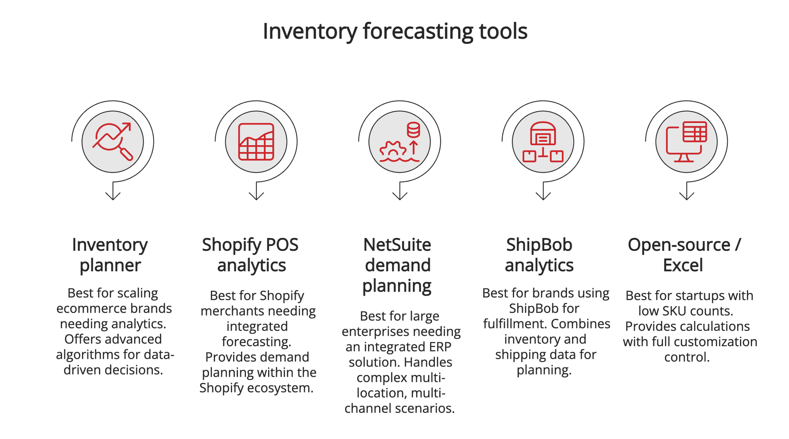
Inventory planner
Best for: Scaling ecommerce brands needing deep analytics and demand planning capabilities. Offers advanced forecasting algorithms and detailed reporting for data-driven decision making.
Shopify POS analytics
Best for: Shopify merchants who need basic, integrated forecasting without additional software costs. Provides essential demand planning within the familiar Shopify ecosystem.
Maximize your Shopify forecasting by partnering with the best 3PL for Shopify to combine platform data with fulfillment expertise.
NetSuite demand planning
Best for: Large enterprises needing an integrated ERP solution with comprehensive forecasting capabilities. Handles complex multi-location, multi-channel scenarios.
ShipBob analytics
Best for: Brands using ShipBob for fulfillment who want integrated forecasting software that combines inventory and shipping data for comprehensive planning.
Open-source / Excel template
Best for: Startups and businesses with low SKU counts who need basic forecasting without monthly software costs. Provides essential calculations with full customization control.
Real-world case study: Adventure gear retailer
An adventure gear retailer constantly faced stockouts of their best-selling hiking boots while being overstocked on slow-moving winter tents. This classic inventory imbalance was costing them customers and tying up precious working capital.
The challenge: Poor demand visibility led to reactive ordering decisions that created a cycle of stockouts on popular items and excess inventory on seasonal products.
The approach: They implemented a quantitative inventory forecasting model using EOQ calculations to right-size orders and added safety stock buffers to protect against supplier delays and demand variability.
The results: Within six months, they reduced stockouts from 25% to 10%, cut storage costs from $8,000/month to $5,000/month, and doubled their inventory turnover. Most importantly, customer satisfaction improved significantly as popular products stayed in stock consistently.
This transformation demonstrates how systematic inventory forecasting delivers measurable results when properly implemented with commitment to data quality and process discipline.
ALERT: Success requires consistent execution over time. The retailer achieved these results by tracking forecast accuracy weekly and adjusting their approach based on real performance data.
Common mistakes & how to avoid them
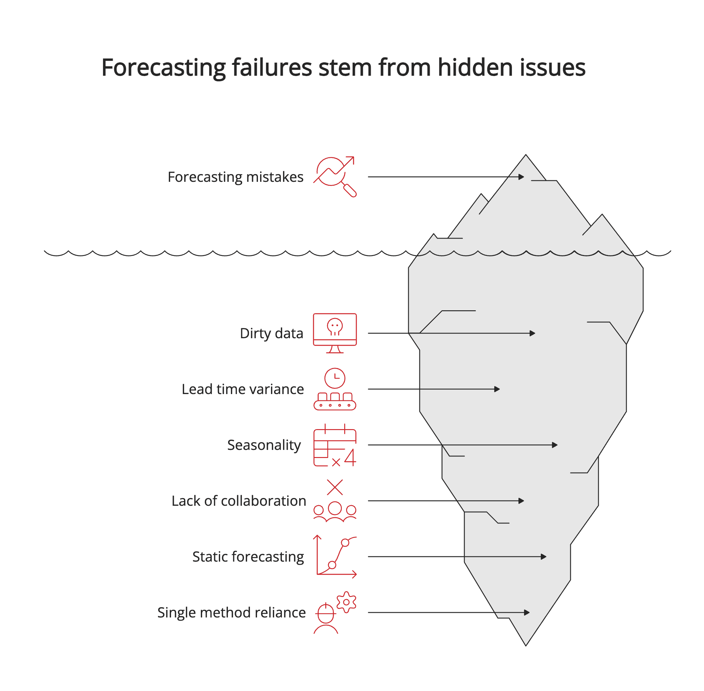
Even sophisticated forecasting efforts can fail due to common pitfalls that undermine accuracy and reliability. Learning from these mistakes accelerates your path to forecasting success.
Using ‘dirty’ or incomplete data: Clean, consistent data is non-negotiable for accurate forecasts. Remove anomalies and ensure data quality before any analysis.
Ignoring lead time variance: Average lead times mask dangerous variability. Track minimum, maximum, and standard lead times to build appropriate buffers.
Forgetting seasonality and promotions: Historical patterns include seasonal and promotional spikes. Account for these factors in your future projections.
Not collaborating with marketing & sales: Forecasting in isolation misses critical business intelligence. Include promotional calendars and sales insights in your models.
‘Set it and forget it’ forecasting: Markets change constantly. Review and update forecasts regularly based on actual performance and changing conditions.
Relying on a single forecasting method: No single approach works for all situations. Combine multiple methods for more robust predictions.
Following inventory forecasting best practices means building systematic processes that improve over time rather than seeking perfect accuracy immediately.
Frequently asked questions
Here are direct answers to the most common questions about inventory forecasting.
What is inventory forecasting in supply chain management?
Inventory forecasting in supply chain management is the process of predicting inventory needs to balance supply and demand across the entire supply chain network. It coordinates raw materials, work-in-progress, and finished goods to optimize flow and minimize costs.
How do you calculate an inventory forecast?
Calculating an inventory forecast involves gathering historical sales data, determining key metrics like lead time, demand, and safety stock, and then applying a forecasting method like time-series analysis or EOQ calculations. The specific formula depends on your chosen approach and business requirements.
What are the 4 types of inventory forecasting?
The four main forecasting methods are: Trend forecasting (using historical patterns), Graphical forecasting (visual data analysis), Qualitative forecasting (expert opinion and market research), and Quantitative/time-series forecasting (statistical models and algorithms).
Which formula is used to calculate safety stock?
The standard safety stock formula is: (Max daily sales × Max lead time) - (Avg daily sales × Avg lead time). This calculation provides a buffer against demand variability and supply disruptions.
How do I calculate inventory forecast accuracy?
The most common accuracy measurement uses Mean absolute percentage error (MAPE): MAPE = (|Actual sales - Forecasted sales| / Actual sales) × 100. Track this metric over time to improve your forecasting performance.
Citations
- Slimstock. “The Hidden Cost of Stockouts.” 2025.
- Flieber. “Stockout Costs.” 2025.
- Zoho. “Inventory Carrying Cost.” 2024.
- eCampusOntario. “Seasonal Indices.” 2025.
- Based on internal analysis and common industry results.
- Standard industry formula for Mean Absolute Percentage Error (MAPE).
